PCB Tech - Analyze characteristic impedance

In recent years, an increasingly important issue in the field of high-speed design is the design of circuit boards with controlled impedance and the characteristic impedance of interconnect lines on the circuit board. However, for non-electronic design engineers, this is also the most confusing and least intuitive problem. Even many electronic design engineers are equally confused about this. This information will give a brief and intuitive introduction to the characteristic impedance, hoping to help you understand the most basic quality of the transmission line.

What is a transmission line?

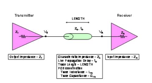
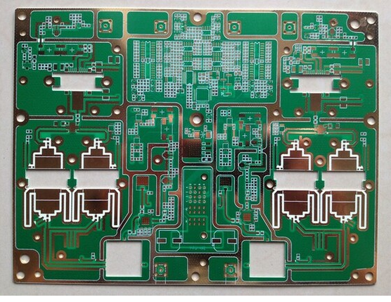
What is a transmission line? Two conductors with a certain length constitute a transmission line. One of the conductors becomes the signal propagation channel, while the other conductor constitutes the signal return path (here we mention the signal return path, which is actually the ground that everyone usually understands, but for the convenience of the description, forget the ground for the time being. The concept.). In a multi-layer circuit board design, each PCB interconnection line constitutes a conductor in the transmission line, and the transmission line uses the adjacent reference plane as the second conductor or signal return path of the transmission line. What kind of PCB interconnection line is a good transmission line? Generally, if the characteristic impedance is consistent everywhere on the same PCB interconnection line, such a transmission line becomes a high-quality transmission line. What kind of circuit board is called a controlled impedance circuit board? A controlled impedance circuit board means that the characteristic impedance of all transmission lines on the PCB meets a unified target specification. It usually means that the characteristic impedance of all transmission lines is between 25Ω and 70Ω.

From the perspective of the signal

The most effective way to consider the characteristic impedance is to look at what the signal itself sees as it propagates along the transmission line. To simplify the discussion of the problem, it is assumed that the transmission line is a microstrip type, and the cross section of the transmission line is consistent when the signal propagates along the transmission line.

Add a step signal with an amplitude of 1V to the transmission line. The step signal is a 1V battery, which is connected by the front end and connected between the signal line and the return path. At the moment when the battery is switched on, the signal voltage waveform will travel in the dielectric at the speed of light, usually at a speed of about 6 inches/ns (why the signal travels so fast, rather than close to the electron propagation speed of about 1cm/s, this is another topic, No further introduction here). Of course, the signal here still has a conventional definition. The signal is defined as the voltage difference between the signal line and the return path, which is always obtained by measuring the voltage difference between any point on the transmission line and the adjacent signal return path.

The signal is forwarded along the transmission line at a speed of 6 inches/ns. What kind of situation will the signal encounter during the transmission? In the first 10ps time interval, the signal traveled a distance of 0.06 inches along the transmission line. Assuming that the lock time is at this moment, consider what happens on the transmission line. Over this distance of travel, the transmission of the signal establishes a stable constant signal with an amplitude of 1V between this section of the transmission line and the corresponding adjacent signal return channel. This means that extra positive charges and extra negative charges have been accumulated on this section of the transmission line and the corresponding return path to establish this stable voltage. It is the difference of these charges that establishes and maintains a stable 1 V voltage signal between the two conductors, and the stable voltage signal between the conductors establishes a capacitance between the two conductors.

The transmission line segment behind the signal wavefront on the transmission line is not clear that there will be a signal to propagate, so the voltage between the signal line and the return path is still maintained at zero. In the next 10ps time interval, the signal will travel a certain distance along the transmission line. As a result of the signal continuing to propagate, a 1V transmission line will be established between another transmission line segment with a length of 0.06 inches and the corresponding signal return path. Signal voltage. In order to do this, a certain amount of positive charge must be injected into the signal line, and the same amount of negative charge must be injected into the signal return path. For every 0.06 inches of signal propagation along the transmission line, more positive charges will be injected into the signal line, and more negative charges will be injected into the signal return path. Every 10ps time interval, another section of the transmission line will be charged to 1 V, and the signal will continue to propagate along the direction of the transmission line.

Where do these charges come from? The answer comes from the signal source, which is the battery we use to provide the step signal and connect to the front end of the transmission line. As the signal propagates on the transmission line, the signal continuously charges the transmission line segment that it propagates through, ensuring that a voltage of 1 V is established and maintained between the signal line and the return path wherever the signal is transmitted. Every 10ps time interval, the signal will travel a certain distance on the transmission line and draw a certain amount of charge δQ from the power system. The battery provides a certain amount of charge δQ to the outside within a period of time δt to form a constant signal current. A positive current flows from the battery into the signal line, and at the same time a negative current of the same magnitude flows through the signal return path.

The negative current flowing through the signal return path is exactly the same as the positive current flowing into the signal line. Moreover, at the position of the signal wavefront, the AC current flows through the capacitor formed by the signal line and the signal return path, completing the signal loop.

Characteristic impedance of transmission line

From the perspective of the battery, once the design engineer connects the lead of the battery to the front end of the transmission line, there is always a constant value of current flowing out of the battery, and the voltage signal is kept stable. Some people may ask, what kind of electronic components have such behavior? When a constant voltage signal is added, it will maintain a constant current value, which is of course a resistance.

As for the battery, when the signal propagates forward along the transmission line, every 10ps time interval, a new transmission line segment of 0.06 inches will be added to be charged to 1V. The newly increased charge obtained from the battery ensures that a stable battery is maintained. The current draws a constant current from the battery, the transmission line is equivalent to a resistor, and the resistance is constant. We call it the surge impedance of the transmission line.

Similarly, when a signal travels forward along a transmission line, every certain distance it travels, the signal will constantly probe the electrical environment of the signal line and try to determine the impedance of the signal when it travels further forward. Once the signal has been added to the transmission line and propagated along the transmission line, the signal itself has been examining how much current is needed to charge the length of the transmission line that propagates in the 10ps time interval, and keep this part of the transmission line segment charged to 1V. This is the instantaneous impedance value we want to analyze.

From the perspective of the battery itself, if the signal propagates along the direction of the transmission line at a constant speed, and assuming that the transmission line has a uniform cross-section, then each time the signal propagates a fixed length (such as the distance the signal propagates in a 10ps time interval), then it needs Get the same amount of charge from the battery to ensure that this section of the transmission line is charged to the same signal voltage. Each time the signal propagates a fixed distance, the same current will be obtained from the battery and the signal voltage will be kept consistent. During the signal propagation process, the instantaneous impedance everywhere on the transmission line is the same.

In the process of signal propagation along the transmission line, if there is a consistent signal propagation speed everywhere on the transmission line, and the capacitance per unit length is also the same, then the signal will always see a completely consistent instantaneous impedance during the propagation process. Since the impedance remains constant on the entire transmission line, we give a specific name to represent this characteristic or characteristic of a specific transmission line, which is called the characteristic impedance of the transmission line. The characteristic impedance refers to the instantaneous impedance value seen by the signal when the signal propagates along the transmission line. If the characteristic impedance seen by the signal remains the same at all times while the signal is propagating along the transmission line, then such a transmission line is called a controlled impedance transmission line.

The characteristic impedance of the transmission line is the most important factor in the design

The instantaneous impedance or characteristic impedance of the transmission line is the most important factor affecting signal quality. If the impedance between adjacent signal propagation intervals remains the same during signal propagation, then the signal can propagate forward very smoothly, and the situation becomes very simple. If there is a difference between adjacent signal propagation intervals, or the impedance changes, part of the energy in the signal will be reflected back, and the continuity of signal transmission will also be destroyed.

In order to ensure the best signal quality, the goal of signal interconnection design is to ensure that the impedance seen by the signal during transmission remains as constant as possible. This mainly refers to keeping the characteristic impedance of the transmission line constant. Therefore, the design and manufacture of PCB boards with controlled impedance becomes more and more important. As for any other design tricks such as minimizing the finger length, terminal matching, daisy chain connection or branch connection, etc., all are to ensure that the signal can see a consistent instantaneous impedance.

Calculation of characteristic impedance

From the above simple model, we can deduce the value of the characteristic impedance, that is, the value of the instantaneous impedance seen during the transmission of the signal. The impedance Z seen by the signal in each propagation interval is consistent with the basic definition of impedance

Z=V/I

The voltage V here refers to the signal voltage added to the transmission line, and the current I refers to the total amount of charge δQ obtained from the battery in each time interval δt, so

I=δQ/δt

The charge flowing into the transmission line (the charge ultimately comes from the signal source) is used to charge the capacitance δC formed between the newly added signal line and the return path in the signal propagation process to the voltage V, so

δQ=VδC

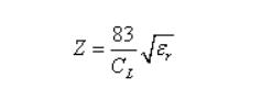
We can relate the capacitance caused by the signal traveling a certain distance during the propagation process with the capacitance value CL per unit length of the transmission line and the speed U of the signal propagating on the transmission line. At the same time, the distance the signal travels is the speed U multiplied by the time interval δt. So

δC = CL U δt

Combining all the above equations, we can derive the instantaneous impedance as:

Z=V/I=V/(δQ/δt)=V/(VδC/δt)=V/(V CL U δt /δt)=1/(CL U)

It can be seen that the instantaneous impedance is related to the capacitance value per unit transmission line length and the speed of signal transmission. This can also be artificially defined as the characteristic impedance of the transmission line. In order to distinguish the characteristic impedance from the actual impedance Z, a subscript 0 is specially added to the characteristic impedance. The characteristic impedance of the signal transmission line has been obtained from the above derivation:

Z0 = 1/(CL U)

If the capacitance value per unit length of the transmission line and the speed at which the signal propagates on the transmission line remain constant, then the transmission line has a constant characteristic impedance within its length. Such a transmission line is called a controlled impedance transmission line.

It can be seen from the above brief description that some intuitive knowledge about capacitance can be connected with the newly discovered intuitive knowledge of characteristic impedance. In other words, if the signal wiring in the PCB is widened, the capacitance value per unit length of the transmission line will increase, and the characteristic impedance of the transmission line can be reduced.

Intriguing topic

Some confusing statements about the characteristic impedance of transmission lines can often be heard. According to the above analysis, after connecting the signal source to the transmission line, you should be able to see a certain value of the characteristic impedance of the transmission line, for example, 50Ω. However, if you connect an ohmmeter to the same 3-foot-long RG58 cable, The measured impedance is infinite.

The answer to the question is that the impedance value seen from the front end of any transmission line changes with time. If the time for measuring the cable impedance is short enough to be comparable to the time the signal takes to go back and forth in the cable, you can measure the surge impedance of the cable or the characteristic impedance of the cable. However, if you wait for enough time, a part of the energy will be reflected back and detected by the measuring instrument. At this time, the impedance change can be detected. Normally, in this process, the impedance will change back and forth until the impedance value. A stable state is reached: if the end of the cable is open, the final impedance value is infinite, and if the end of the cable is short-circuited, the final impedance value is zero.

For a 3-foot-long RG58 cable, the impedance measurement process must be completed within a time interval of less than 3ns. This is what the Time Domain Reflectometer (TDR) will do. TDR can measure the dynamic impedance of a transmission line. If it takes a time interval of 1s to measure the impedance of a 3-foot-long RG58 cable, then the signal has been reflected back and forth millions of times during this time interval, then you may get completely different from the huge change in impedance The value of impedance, the final result is infinity, because the terminal of the cable is open.