
With the ever-faster edges of signals, the problems faced by designers of today's high-speed digital PCB board were unimaginable a few years ago. For signal edge changes of less than 1 nanosecond, the voltage between the power supply layer and the ground layer on the PCB is not the same everywhere on the circuit board, which affects the power supply of the IC chip and causes the logic error of the chip. To ensure the correct operation of high-speed devices, designers should eliminate such voltage fluctuations and maintain low-impedance power distribution paths. To do this, you need to add decoupling capacitors to the circuit board to reduce the noise generated by high-speed signals on the power and ground planes. You have to know how many capacitors to use, what the value of each capacitor should be, and where to put them on the board. On the one hand, you may need a lot of capacitors, and on the other hand, the space on the circuit board is limited and precious, and these details can make or break the design.

The trial-and-error design approach is time-consuming and expensive, often resulting in over-constrained designs that add unnecessary manufacturing costs. Using software tools to simulate and optimize board designs and board resource usage is a more practical approach for designs that are iteratively tested for various board configurations. This article illustrates this process using the design of an xDSM (Dense Subcarrier Multiplexing) circuit board for a fiber/broadband wireless network. The software simulation tool uses Ansoft's SIwave, which is based on hybrid full-wave finite element technology and can import board designs directly from layout tools Cadence Allegro, Mentor Graphics BoardStation, Synopsys Encore, and Zuken CR-5000 Board Designer. Figure 1 is the PCB layout of the design in SIwave. Since the structure of the PCB is planar, SIwave can efficiently perform a comprehensive analysis, and its analysis output includes the board's resonance, impedance, S-parameters of the selected network, and the equivalent Spice model of the circuit. The dimensions of the xDSM board, ie the power and ground planes, are 11 x 7.2 inches (28 x 18.3 cm). The power and ground layers are both 1.4mil thick copper foils separated by a 23.98mil thick substrate. To understand the design of the board, first, consider the bare-board (no component mounted) characteristics of the xDSM board. Depending on the rise time of high-speed signals on the board, you need to understand the behavior of the board in the frequency domain up to 2GHz. Figure 2 shows the voltage distribution when a sinusoidal signal excites the board to resonate at 0.54GHz. Likewise, the board resonates at 0.81GHz and 0.97GHz and above. For a better understanding, you can also simulate the distribution of the voltage between the power and ground planes in resonant mode at these frequencies.
In resonant mode at 0.54GHz, the voltage difference between the power plane and the ground plane at the center of the board changes to zero. The same is true for some higher frequency resonant modes. But this is not the case in all resonant modes, for example in higher order resonant modes at 1.07GHz, 1.64GHz, and 1.96GHz, the voltage difference variation at the center of the board is non-zero. Finding the point of zero dropout change helps us place devices that require large current changes in a short period of time. For example, if a Xinlix FPGA chip were to be placed on a circuit board, the chip would produce a 2A change in input current in 0.2 nanoseconds. Such a large current change in a short period of time will bring about the power integrity problem of the circuit board, which will cause the circuit board to produce various modes of resonance, resulting in uneven voltages on the power supply layer and the ground layer. However, some resonant modes have zero dropout characteristics at the center of the board, so placing the FPGA chip here avoids these low-frequency resonant modes on the board. The FPGA chip cannot excite these low-frequency resonant modes because coupling to these resonant modes from the center of the board will not be possible. The purple curve shows the resonance caused when the chip at the center of the board draws current from the power plane. In fact, the peaks appear at the higher-order resonant frequencies 1.07GHz, 1.64GHz, and 1.96GHz, but not at the lower-order resonant frequencies 0.54GHz, 0.81GHz, and 0.97GHz, as we expected. The purple curve shows the resonance caused when the chip at the center of the board draws current from the power plane; the green curve shows the response when the chip is placed off-center.
Although device placement and placement can help reduce power integrity problems, they do not solve all problems. First, you can't put all the critical components in the center of the board. Typically, device placement flexibility is limited. Second, there are always some resonant modes that will be excited at any given location. For example, the green curve in Figure 3 shows that when you place the chip off-center along some axis, the 0.54GHz resonant mode will be excited. The key to successfully designing a circuit board's PDS (power distribution system) is to add decoupling capacitors at appropriate locations to ensure the integrity of the power supply and to ensure that the ground bounce noise is small enough over a wide enough frequency range.
Decoupling capacitor
Imagine an FPGA sinking 2A on a 0.2ns rising edge, at which point the supply voltage is temporarily lowered (dropout) and the ground plane voltage is temporarily pulled up (ground bounce). The magnitude of its variation depends on the impedance of the board and the decoupling capacitors at the chip bias pins for supplying current (Figure 4a). Since the transient value of the current is 2A, the transient value of the voltage is determined by V=Z×I, Z is the impedance seen from the chip end, therefore, in order to avoid the peak fluctuation of the voltage, in the frequency range from DC to the signal bandwidth, the Z value must be below a certain threshold. The magnitude of its variation depends on the impedance of the board and the decoupling capacitors at the chip bias pins for supplying current; in order to avoid voltage spikes, the Z value must be below a certain frequency in the frequency range from DC to the signal bandwidth. a threshold value. The dotted line part in the figure is the target area that the PDS impedance should meet. In this design, to maintain power integrity, power-to-ground voltage fluctuations must be kept within 5% of the standard value of 3.3V. Therefore, the noise cannot be greater than 0.05×3.3V=165 mV. According to this, the impedance of PDS can be calculated according to Ohm's law: 165mV/2A=82.5mΩ
. For frequencies, usually 1 kHz or lower - the power supply meets the impedance characteristics, and the structure of the power supply and ground planes usually do not destroy the impedance characteristics because they exhibit low resistance and inductance characteristics. And when the frequency is higher than 1kHz, the mutual inductance of the current path is large enough to cause the voltage to exceed the limit value, according to For higher frequencies, the decoupling capacitor is necessary as a low impedance connection between the power plane and the ground plane. The signal bandwidth required to meet the PDS impedance requirements can be estimated by the following equation: In this design, its bandwidth is 1.75GHz.
In order to achieve such a wide bandwidth, it is usually necessary to place many high-frequency ceramic capacitors in the MHz signal area and place larger electrolytic capacitors in the kHz signal area. Together with other components, these capacitor matrices take up valuable board space. Physical prototypes are indispensable in trial-and-error design methods, and virtual prototyping technology allows designers to solve this problem without the need for physical prototypes. Designing a PDS for a PCB board, such as the xDSM board in this example, uses SIwave to place a port at the IC chip and calculate the board's input impedance within the appropriate bandwidth. The red curve in Figure 5 shows the impedance with no capacitors on the board. Both the impedance axis and the frequency axis take logarithmic coordinates. The simulation shows the effect of the capacitance of the board itself and ignores the low induced current loop through the power supply. As you can see from the graph, the impedance increases with decreasing frequency, but since the loop through the power supply also has low impedance, this relationship is not strict. The red curve shows the impedance when there is no capacitor on the circuit board; the dark blue curve is the impedance characteristic after redesign; the light blue curve is the impedance curve after adding a 10nF capacitor matrix; the colored curve shows the 1nF capacitor matrix is added again. the result of. According to Z=1/(j·C), the straight line in the red curve shows that the capacitance of the board itself is 74nF. To keep the impedance below the target impedance of 82.5mΩ at 1MHz, the capacitor value should be at least 2µF—almost 30 times the capacitance of the board itself. For this, 22 0.1μF capacitor matrices need to be added first. The dark blue curve in the figure is the redesigned impedance characteristic. In most frequency ranges, the design meets the requirements of impedance characteristics. But at the high end of the bandwidth, the capacitor's ESL (equivalent series inductance), ESR (equivalent series resistance), and the additional inductance caused by the capacitor spacing make the impedance curve not meet the impedance characteristic requirements. Since smaller capacitors have smaller ESL and ESR values, adding bypass helps to improve their high-frequency characteristics. The light blue curve in Figure 5 is the impedance curve after adding another 10nF capacitor matrix. The green curve shows the result after adding the 1nF capacitor matrix again. The addition of each capacitance matrix improves the impedance characteristics, but the result is still just enough to meet the impedance characteristics. At this stage of the design, the designer can add electromagnetic simulation along with circuit simulation to complete the design. This approach allows designers to model low-side impedances, including power supply loading effects. It can also directly stimulate the noise on the power pins to directly verify the power plane noise, avoiding unnecessary design overhead caused by excessive analysis of the power plane impedance.
The input and output ports should first be added at the selected locations. The port has been added at one IC chip above, and then a port should be added at the power input end, and two ports should be added at the mounting position of the other two chips. Then in SIwave, you can do a broadband sweep to get a 4x4 S-parameter scattering matrix over the entire bandwidth. Full-Wave Spice can then be used to generate Spice-compatible circuit files for further analysis in the circuit simulation environment. In the generated circuit file, the PCB board is in the center of the circuit. The circuit file also includes a model of the FPGA - a current source with a current probe and a differential voltage probe. The Spice circuit created by Full-wave Spice also includes the three capacitor matrices mentioned above. Adding a fourth capacitor matrix at the IC will further reduce the high-side impedance. The circuit also includes a DC power supply with a small amount of decoupling capacitors ranging from 1nF to 100µF. Also included are models of two other IC chips, surrounded by a small array of 100nF capacitors.
The blue and green curves represent the power integrity curves of the IC chip without adding and adding a set of capacitor matrices, respectively; the red curve represents the sudden change of the chip's input current. Noise simulation results for the power supply voltage of the FPGA are shown. The red curve represents a sudden change in the chip's input current - the current changes from 0A to 2A in 0.2 nanoseconds. The blue curve represents the voltage curve of the IC chip without adding a set of capacitor matrices. Compared to 3.3V, the voltage fluctuation is already very small, but it still exceeds the 5% specification. The green curve represents the voltage fluctuation curve after adding the fourth group of capacitor matrix, and the final design meets the specification that requires that the power supply noise is less than 165mV. The other chips on the board can be analyzed in the same way to ensure that they are not affected by power drops and ground bounces. In this example, the other two chips draw 100mA and 50mA respectively, and their contribution to noise is relatively small. PCB board-level design of high-speed circuits is very challenging. In order to ensure the correct operation of the circuit, the PDS of the circuit needs to be carefully designed, including adding hundreds of decoupling capacitors on the circuit board and choosing the appropriate capacitor value and location according to the needs. Using the simulation method of virtual prototype instead of the trial and error design method to optimize the power integrity design of the PCB board can effectively shorten the design cycle and save the design cost.